Introduction and Motivation
The Neural Turing Machine (NTM) (Graves, Wayne, and Danihelka 2014) is a memory-augmented neural network architecture introduced by Alex Graves and colleagues from DeepMind in 2014. Although its architectural components are loosely inspired by Alan Turing’s Turing Machine, Graves later mentioned during a lecture that the metaphor has become somewhat strained and perhaps “Neural Von Neumann Machine” would have been a more fitting name as the key idea of the architecture is to decouple memory from computation (Graves 2018). Similar to a CPU interacting with the RAM, a controller network learns to perform read/write operations on a large external memory matrix. This separation aims to alleviate a shortcoming of commonly used recurrent networks, namely that their computational complexity grows exponentially as the hidden state’s capacity is increased. The second important contribution of the paper was its novel use of soft attention mechanisms to index discrete memory locations. Ubiquitous today, attention can be used to make all memory interactions differentiable. This makes the NTM trainable end-to-end using the backpropagation algorithm. The result is an expressive architecture that is capable of learning simple algorithms from input-output-samples. Or framed differently, a differentiable computer, that programs itself based on inputs from its environment. The original paper showed that the NTM outperforms Long Short-Term Memory Networks on a range of memory tasks.
Since the NTM was published different variations have been proposed and new memory-augmented architectures have been developed. Furthermore, over the years these architectures have found their way into the artificial brains of agents in various reinforcement learning settings. In spite of the bells and whistles proposed by newer architectures, I think the Neural Turing Machine remains a great introduction to neural memory mechanisms. The paper is very accessible and introduces important aspects and primitives to think about, such as associative recall and how attention can be used for operating on discrete data-structures in a differentiable manner.
My main goal for this post is to explain the NTM architecture using a bottom-up approach. I will begin each section by going through the theory and the mathematical formulations. I tried to include visual examples to help the reader build an intuitive understanding of the different memory operations. Each theory section is followed by a code interlude, in which we will implement what we have learned using the Pytorch library. By the end of this post, we will have created a working implementation of the Neural Turing Machine. I will conclude with addressing some of the architecture’s shortcomings and present some tricks that can help to stabilise the training process.
The implementation was inspired by existing open source repositories (Ha 2017; Zana 2017). I adopted the modular style, the HeadBase class for shared functionality between heads, the learned initialisation strategy, as well as the hidden state unpacking scheme. I tried to simplify the way a module’s parameters and/or state can be initialised and reset. By introducing appropriate methods for this purpose, it becomes easier to experiment with different initialisations, which, as we will see later, turns out to be essential to make the training process numerically stable.
Architecture Overview
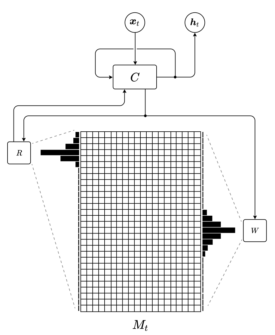
Figure 1: Schematic of the Neural Turing Machine architecture.
Figure 1 shows the main components of the Neural Turing Machine. It is comprised of a controller network \(C\) (usually a recurrent model such as an LSTM, but feed-forward is also possible), a memory matrix \(M\) and a set of read and write heads, \(R\) and \(W\). At each time step \(t\), the controller receives an input \(\boldsymbol{x}_t\) from the environment. Using the current input and its previous state \(\boldsymbol{h}_{t-1}\), it then produces parameters or instructions for the heads. By following these instructions, a head’s current focus is shifted to specific rows or slots of the memory matrix and a read or write operation is executed. Finally, The read-out vectors are routed back to the controller, where they are incorporated into the new state \(\boldsymbol{h}_{t}\) and the final output is generated.
In the following sections we will explore in detail how the read and write operations are defined and how each head produces its attention vector.
Reading and Writing
Based on the instructions it receives from the controller, a head selects one or more memory locations for reading or writing by attending to the slots in memory to varying degrees1. A head can thereby focus sharply on the memory at a single location or weakly at many locations.
How exactly this attention mechanism works will be discussed in detail in the Section on memory addressing. Before that, we will take a look at the mathematical operations that underlie the reading and writing processes.
Reading
Assume that at a given time step \(t\), we have a read head \(R\) and a memory \(M_t\). In our example, the memory has 4 distinct memory slots, each of which stores a 5-dimensional binary vector2. Based on the current input from the controller the read head produces a normalised attention vector \(\boldsymbol{w}^\text{r}_t\) with values between 0 and 1 and a total sum equal to 1. The head determines thereby how much focus should be given to each of the memory’s locations.
Using these weightings, we can define a reading procedure that reads a vector \(\boldsymbol{r}_t\) from memory:
\[ \begin{equation} \boldsymbol{r}_{t} = \sum_{i} \boldsymbol{w}^\text{r}_{t}(i) M_{t}(i) \end{equation} \]
This operation can be visualized in two steps. First, each element of the focus vector \(\boldsymbol{w}^\text{r}_t\) is multiplied with the corresponding row in memory. Second, the rows are added together to produce the read vector \(\boldsymbol{r}_t\):
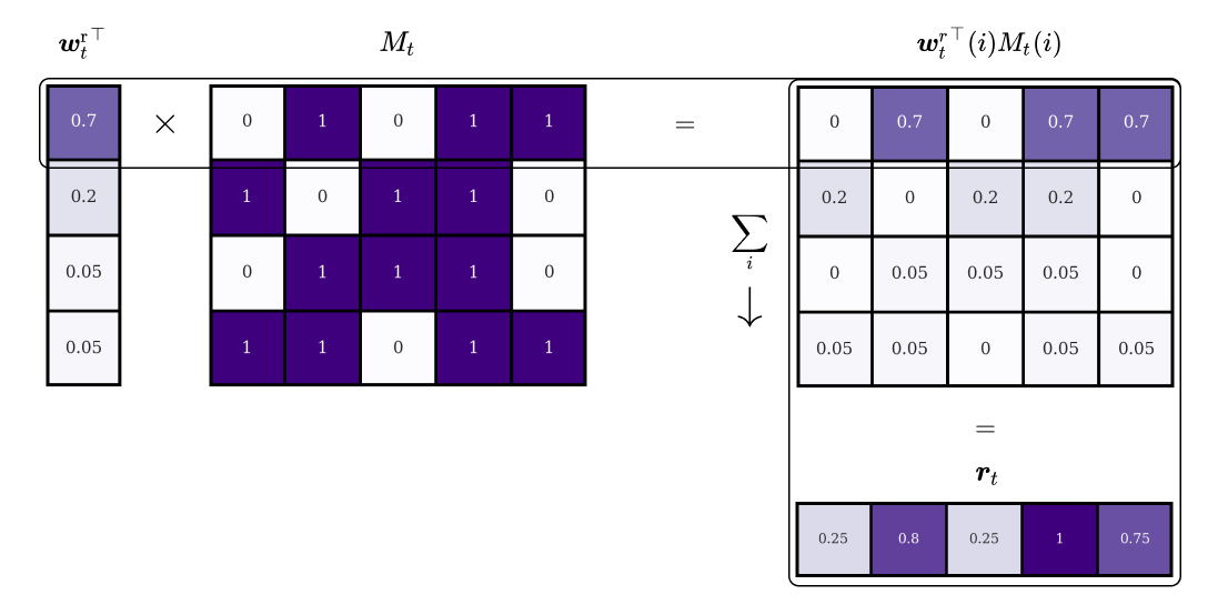
The resulting read vector is simply a weighted sum of the contents of the locations.
Now let’s see how information can be written to the memory.
Writing
Inspired by Long Short Term Memory networks (with forget gates), the writing operation is decomposed into two steps: erase and add. At any given time step \(t\), we have a write head \(W\) with attention weightings \(\boldsymbol{w}^\text{w}_t\) and a memory matrix from the previous time step \(M_{t-1}\). Before we can delete information, we need to determine to which degree each of the stored elements should be erased. For this purpose, we introduce the erase vector \(\boldsymbol{e}_t\) with the same dimensions as a single memory location and values in the range \([0, 1]\). Each element corresponds to a cell in a given location and indicates how many per cent of the cell’s value should be erased. For example, if an element in \(\boldsymbol{e}_t\) has the value \(1\), the corresponding cell value in the memory location will be completely removed. By multiplying the transpose of the weightings with the erase vector we obtain a matrix with the same dimensions as our memory (in our example \(4 \times 5\)):
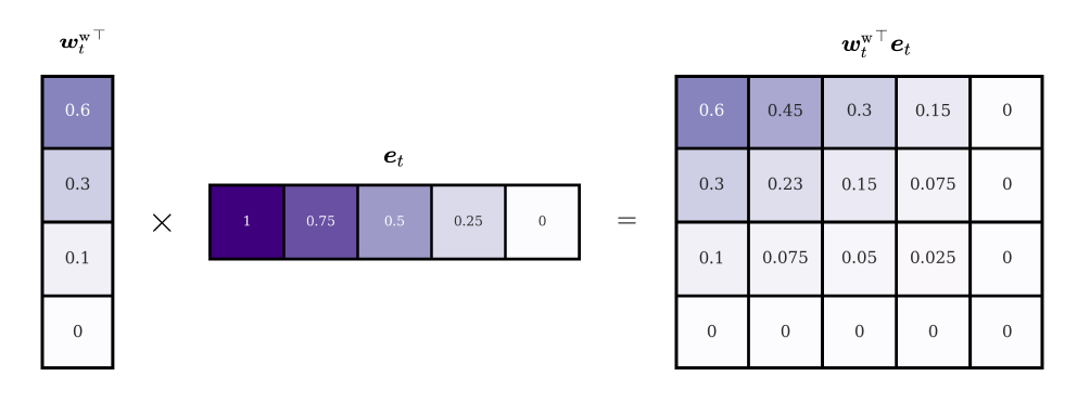
Each row of the resulting matrix represents a different version of the original erase vector, scaled by the head’s attention value at that location3. We can interpret this matrix as an erase filter. Its contents describe how many per cent of a given memory cell should be removed. By subtracting it from a second matrix \(E\) of ones we turn it into a remain filter with the opposite effect.
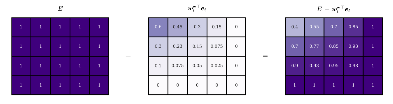
To conclude the erase step, we simply calculate the element-wise product between our filter and the memory of the previous time step:
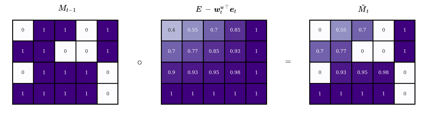
Mathematically, we can express the above steps with the following equation, where \(\tilde{M}_{t}\) is the erased memory matrix:
\[\tilde{M}_{t} = M_{t-1} \circ \left[E-{\boldsymbol{w}_t^\text{w}}^{\top} \boldsymbol{e}_t\right]\]
The next step in the writing process is to generate the information with which the old memory should be updated. To achieve this, we introduce a real-valued add vector \(\boldsymbol{a}_t\) and again multiply it with the transpose of the attention vector. This operation produces an update matrix:
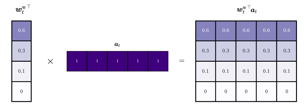
Again, each row of the matrix represents a different version of the original add vector, scaled by the head’s attention value at that location. Finally, the writing operation is completed by adding the update matrix to the erased memory:
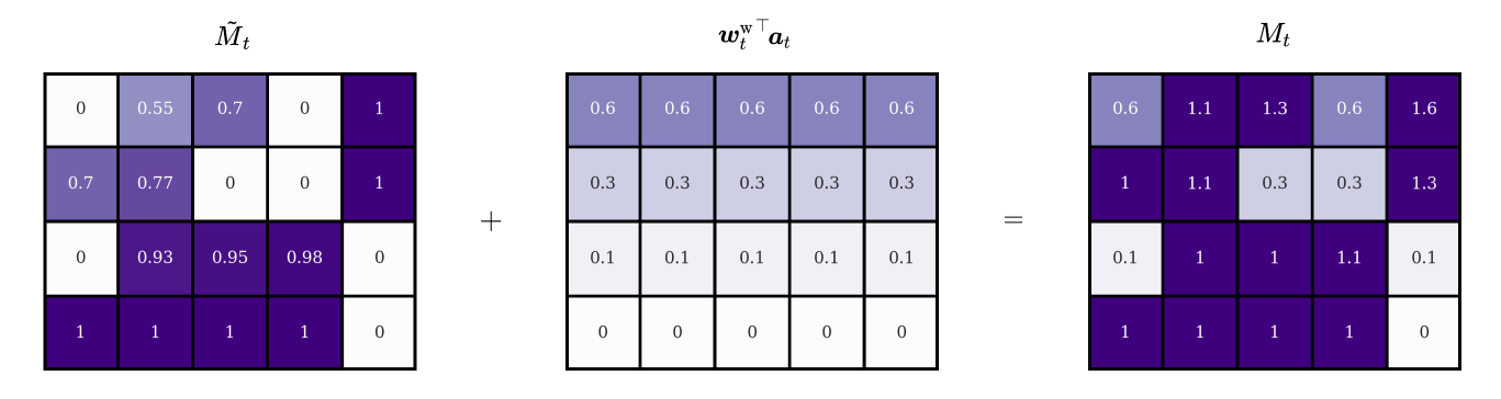
The full writing process can be expressed with the following set of equations:
\[ \begin{align} \tilde{M}_{t} &= M_{t-1} \circ \left[E-{\boldsymbol{w}_t^\text{w}}^{\top} \boldsymbol{e}_t\right]\\ M_t &= \tilde{M}_{t} + {\boldsymbol{w}_t^\text{w}}^{\top} \boldsymbol{a}_t \end{align} \] or more compactly:
\[ M_t = M_{t-1} \circ \left[E-{\boldsymbol{w}_t^\text{w}}^{\top} \boldsymbol{e}_t\right]+ {\boldsymbol{w}_t^\text{w}}^{\top} \boldsymbol{a}_t \]
Interlude: Memory, Reading and Writing in Pytorch
We begin our Neural Turing Machine implementation with the memory module and the reading and writing mechanisms.
We will make use of the following imports:
import torch
from torch import nn
import torch.nn.functional as F
from collections import namedtuple
from torch.nn.utils import clip_grad_norm_
Memory
The memory inherits from nn.Module and is defined by the number of rows, the number of columns and the actual data. The memory contents are represented as a 3-dimensional tensor with shape (batch_size, num_rows, num_columns). In addition, we define an init_state function that can be used to initialise or reset the memory bank. It will be called when the Neural Turing Machine module is instantiated or reset.
class Memory(nn.Module):

    def __init__(self, num_rows, num_cols):
        super(Memory, self).__init__()

        self.num_rows = num_rows
        self.num_cols = num_cols
        self.data     = None

    def init_state(self, batch_size, device):
        self.data = torch.zeros(batch_size, self.num_rows, self.num_cols).to(device)
Reading
Let’s now move to the head implementations. Note that both read and write heads inherit from the HeadBase class, which in turn inherits its traits from nn.Module. For now, it is only important to know that the HeadBase class contains functionality that is shared between both read and write heads e.g. addressing mechanisms (covered in the next section).
In order to implement the read operation a read head needs access to two parameters: the weightings w and the memory contents. While w is passed as an argument from outside, the memory bank is accessed via the memory attribute. w is defined as a tensor of shape (batch_size, num_rows).
class ReadHead(HeadBase):

    def __init__(self, memory):
        super(ReadHead, self).__init__(memory)

    def read(self, w):
        return torch.matmul(w.unsqueeze(1), self.memory.data).squeeze(1)
Writing
The write method takes weightings w, erase vectors e and add vectors a as input and updates the memory contents. Both e and a are defined as tensors of size (batch_size, num_columns).
class WriteHead(HeadBase):

    def __init__(self, memory):
        super(WriteHead, self).__init__(memory)

    def erase(self, w, e):
        return self.memory.data * (1 - w.unsqueeze(2) * e.unsqueeze(1))

    def write(self, w, e, a):
        memory_erased    = self.erase(w, e)
        self.memory.data = memory_erased + (w.unsqueeze(2) * a.unsqueeze(1))
Memory Addressing
At this point, we have seen the mathematical definitions and one possible implementation of the reading and writing operations. One essential question remains to be answered though. How can a head select discrete memory locations in a differentiable manner? The solution to this problem is arguably the key innovation of the Neural Turing Machine architecture. It should be clear from previous sections, that the authors re-framed the discrete indexing problem as one of attention. Under this view, we are now looking for a function that takes parameters (instructions) generated by the controller as input and produces a categorical distribution over all memory locations. The Neural Turing Machine implements this function by combining two complementary addressing mechanisms: content-based and location-based addressing.
Content-based or associative addressing means, that memory locations are selected, whose contents are the most similar to a key vector produced by the controller. Location-based addressing allows a head to shift its current focus to adjacent memory slots within a specified range.
Figure 2 shows the 4-step pipeline implemented by each head to map controller outputs to attention vectors. Each sub-step yields intermediate weightings \(\boldsymbol{w}\).
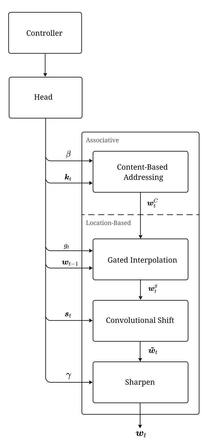
Figure 2: Neural Turing Machine Memory Addressing Pipeline.
Content-based addressing
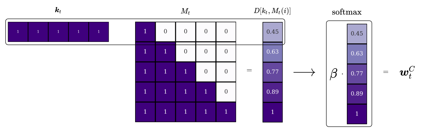
The first step is content-based addressing. The result is an attention vector \(\boldsymbol{w}_t^C\) termed the content-weightings. The focus is strongest for locations, whose contents are the most similar to the current input, or the key, as measured by the cosine similarity \(D\) between the two vectors:
\[D[\mathbf{u}, \mathbf{v}]=\frac{\mathbf{u} \cdot \mathbf{v}}{\|\mathbf{u}\| \cdot\|\mathbf{v}\|}\]
Similarity in the context of the cosine distance means that the cosine of the angle between two given vectors is small. This variable can take on the value 1 (if the vectors point in the same direction), -1 (if the vectors point in perfectly opposite directions) or any value in between (any other angle). For example, let’s say we have the following key \(\boldsymbol{k}\) and memory matrix \(M\). Comparing the key to each entry in the memory yields a similarity vector.
To attenuate or amplify the focus, the similarity vector is multiplied by a real-valued, positive scalar \(\beta\), which we call the key strength.
Finally, to convert the scaled similarity vector into attention weightings we simply apply the softmax function.
We can visualize how the similarity values behave as the key-strength \(\beta\) is increased:
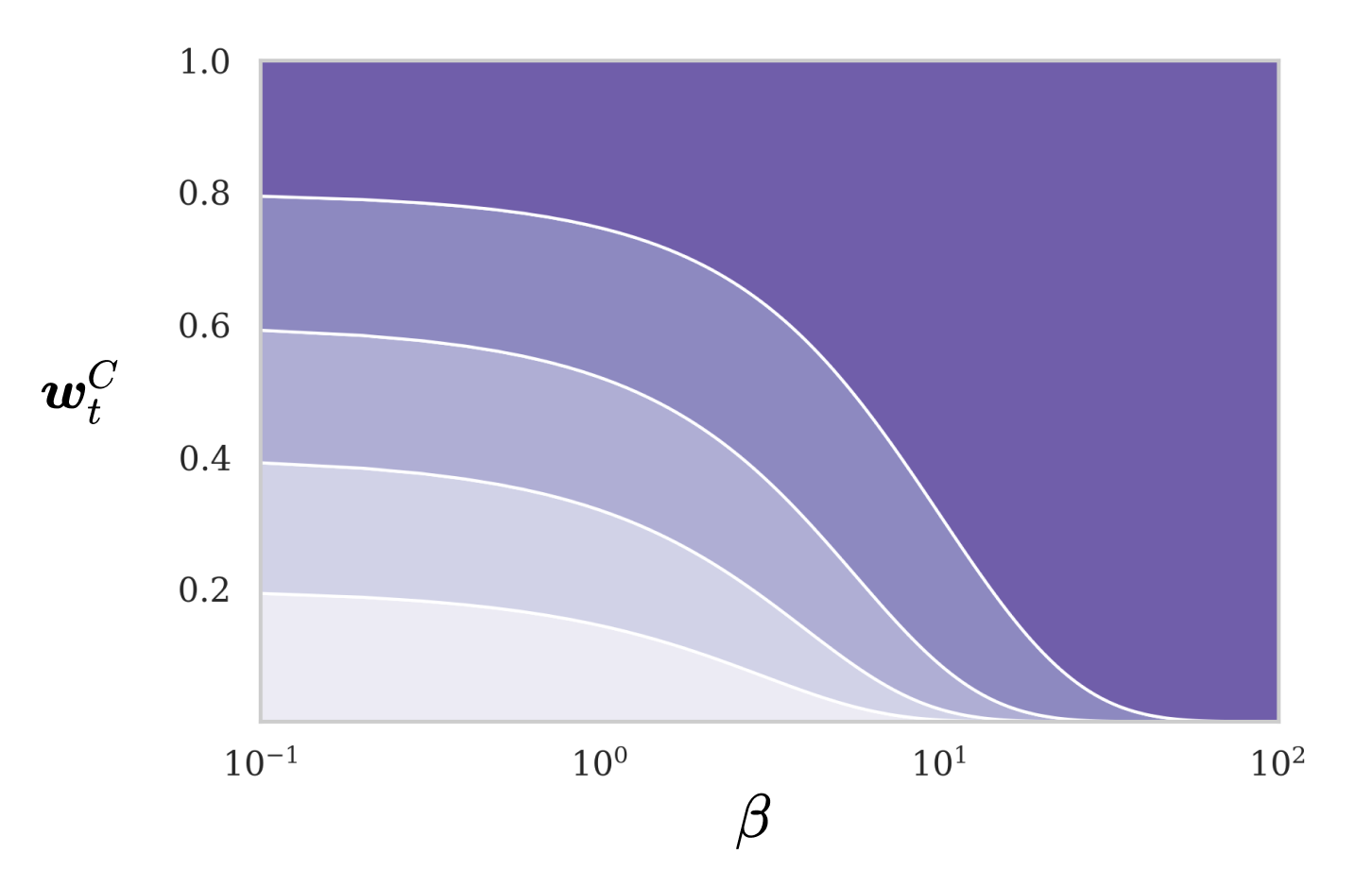
We can observe that for small values of \(\beta\) the focus vector will be diffuse and for large values, the vector will be sharply focused on the row that is most similar to the key.
The main advantage of content-based addressing is how simple it is to retrieve information from memory. The controller merely needs to produce an approximation to the exact, stored item. There are situations, however, where the specific location is more important than the memory contents themselves. This brings us to location-based addressing. But first, let’s take a look at how content-based addressing can be realized in Pytorch.
Interlude: HeadBase and Content-Addressing
Since memory addressing is shared by read as well as write heads, the addressing mechanisms will live inside the HeadBase class. The focus_head method will contain the entire memory addressing pipeline (see Figure 2) to produce the weightings for the current time step. Up until this point, however, we have only seen content-based addressing, which is implemented by the _content_weight method. Its parameters are a batch of keys k of size (batch_size, num_columns) and key strengths of size (batch_size, 1).
class HeadBase(nn.Module):

    def __init__(self, memory):
        super(HeadBase, self).__init__()

        self.memory = memory

        self.init_params()

    def focus_head(self, k, beta):
        w_c = self._content_weight(k, beta)
        return w_c

    def _content_weight(self, k, beta):
        k = k.unsqueeze(1).expand_as(self.memory.data)
        similarity_scores = F.cosine_similarity(k, self.memory.data, dim=2)
        w = F.softmax(beta * similarity_scores, dim=1)
        return w

    def forward(self, h):
        raise NotImplementedError

    def init_state(self, batch_size):
        self.batch_size = batch_size

    def init_params(self):
        pass
Location-based addressing
For some computational processes we do not care about the actual stored information but it is crucial to consistently access a specific memory location. For example when we compute a simple function like \(f(x, y) = xy\) we are indifferent about the actual values of \(x\) and \(y\), but the variables need to be accessed at consistent locations in memory. For this purpose, we implement a mechanism that enables the Neural Turing Machine to shift its heads to specific memory slots, that lie within a given shift-range from its current position. Sequential shifts at each time step allow the network to implement basic looping constructs.
As shown in Figure 2, the addressing mechanism is facilitated by three distinct steps: Gated Interpolation, Convolutional Shift and Sharpen. In the following sections, we are going to look at each of these in separation. As a quick aside before we continue, note that strictly speaking associative addressing is more general than location-based addressing. This is because location information could be stored alongside the actual contents in the memory. In the original paper, however, the authors mentioned that providing location-based addressing as a primitive operation proved essential for some forms of generalisation (Graves, Wayne, and Danihelka 2014).
Gated interpolation
Gated interpolation controls to what extent the content-based addressing mechanism should be used. The controller emits a parameter \(g\) in the range \((0,1)\), which we will call the interpolation gate. Using \(g\), we calculate new weightings as an interpolation between the final attention vector of the previous time step \(\boldsymbol{w}_{t-1}\) and the current content-weightings \(\boldsymbol{w}_t^C\):
\[ \begin{equation} \boldsymbol{w}_{t}^{g} = g_{t} \boldsymbol{w}_{t}^{c}+\left(1-g_{t}\right) \boldsymbol{w}_{t-1} \end{equation} \]
Note that if \(g\) is \(0\) at a given time step the content-weightings \(\boldsymbol{w}_t^C\) will be the zero vector and hence, entirely ignored. Similarly, if \(g\) is \(1\) the weightings of the previous time step \(\boldsymbol{w}_{t-1}\) won’t influence the intermediate weightings \(\boldsymbol{w}_t^g\) for further calculations. If \(g\) is a value between \(0\) and \(1\) exclusive, the two vectors will be blended together in proportion to \(g\).
Convolutional Shift
In this step, we introduce the central mechanism that enables a head to shift its current focus and attend to adjacent memory locations.
The shift operation is implemented as a one-dimensional, circular convolution, where a kernel \(\boldsymbol{s}_t\) emitted by the controller is convolved over the head’s attention vector. \(\boldsymbol{s}_t\) represents a normalised distribution over the allowed integer shifts and you can think of it as shift-instructions. For example, if only shifts by one position are allowed, \(\boldsymbol{s}_t\) will be a vector comprised of three elements, each of which can be interpreted as one of the following instructions:
\[(\texttt{shift 1 forward},\quad \texttt{maintain focus},\quad \texttt{shift 1 backward})\]
Of course, we can have a shift kernel with an allowed shift range greater than one. In the general case, the weightings will have \(2n+1\) elements, where \(n\) is the highest absolute shift value. For instance, for a maximum shift range of two locations, \(\boldsymbol{s}_t\) will now be a \(5\)-dimensional vector:
\[(\texttt{shift +2},\quad \texttt{shift +1},\quad \texttt{shift 0},\quad \texttt{shift -1}\quad \texttt{shift -2})\] The shifted attention vector \(\tilde{\boldsymbol{w}}_{t}\) can be obtained using:
\[ \begin{equation} \tilde{\boldsymbol{w}}_{t}(i) = \sum_{j=0}^{N-1} \boldsymbol{w}_{t}^{g}(j) \boldsymbol{s}_{t}(i-j) \end{equation} \]
First, we unroll the current attention vector \(\boldsymbol{w}_{t}^{g}\) based on the specified maximum shift value in a circular manner. This means, that we append the last element to the beginning and the first element to the end of the sequence. For a maximum shift value \(n > 1\), the sequence is padded with the first \(n\) elements at the tail and the last \(n\) elements at the head. In this way, if a head is focussed on the last row of the memory and performs a forward shift by one position, its focus will move back to the first memory location. Analogously, a backward shift from the first slot, will shift the head’s focus to the end of the memory bank.
Finally, we convolve the shift weightings over the unrolled sequence.
Let’s illustrate this with an example. The maximum shift range is set to 1 position and we have the following attention vector \(\boldsymbol{w}_t^g\) and shift weightings \(\boldsymbol{s}_t\) (note that this filter implements a backward-shift):
Our next step is to pad the sequence in a circular manner. We append the last element to the head and the first element to the tail:
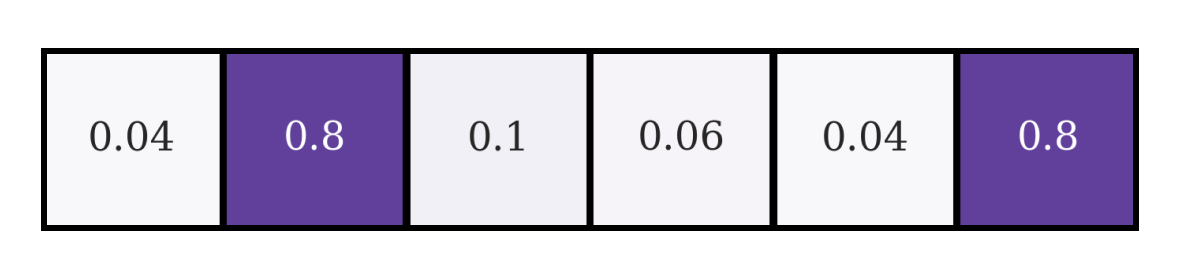
Now we convolve the shift weightings \(\boldsymbol{s}_t\) over the unrolled weightings to calculate the shifted weightings \(\tilde{\boldsymbol{w}}_t\):
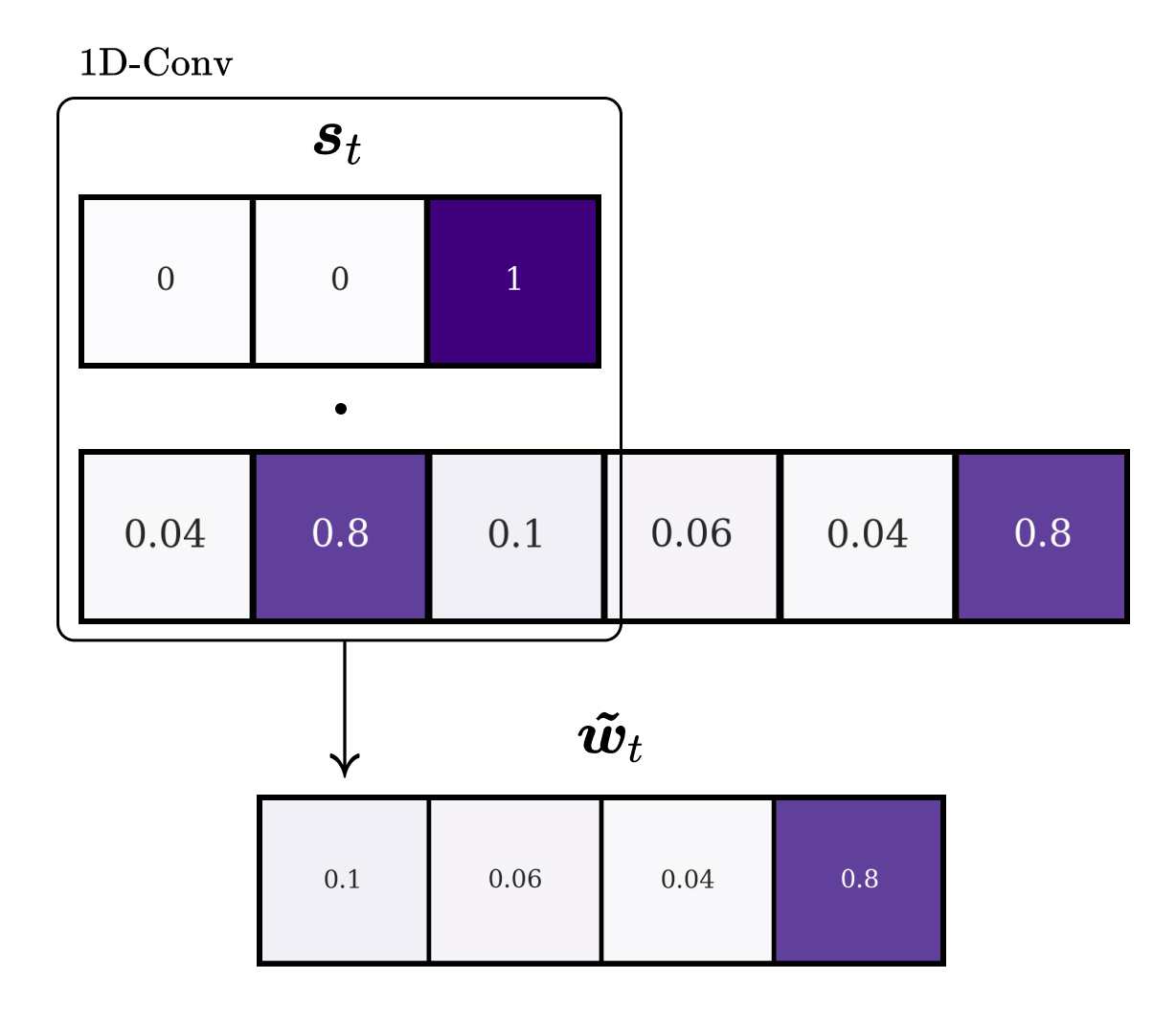
Compare \(\boldsymbol{w}_{t}^{g}\) with \(\tilde{\boldsymbol{w}}_t\). We can observe, that the head’s attention has shifted one position backwards.
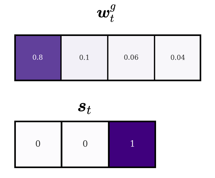
We have seen now how we can leverage the circular convolution operation to shift a head’s focus. There is, however, one more aspect of this implementation that we need to consider. Remember that the shift weightings are a normalised distribution over the possible shift instructions. This distribution, however, does not need to be sharply focussed on only a single instruction. How does an unfocussed shift-kernel shift the attention on the memory locations? Assume that we have a maximum shift range of one, a sharply focussed attention vector \(\boldsymbol{w}^g_t = (1, 0, 0, 0)\) (four memory slots) and slightly dispersed shift weightings \(\boldsymbol{s}_t = (0.7, 0.1, 0.2)\):
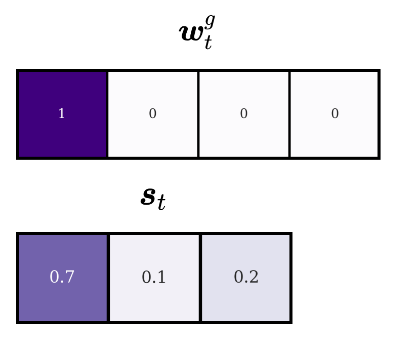
After we apply our shift operation, we obtain the following shifted focus vector \(\tilde{\boldsymbol{w}}_t\):
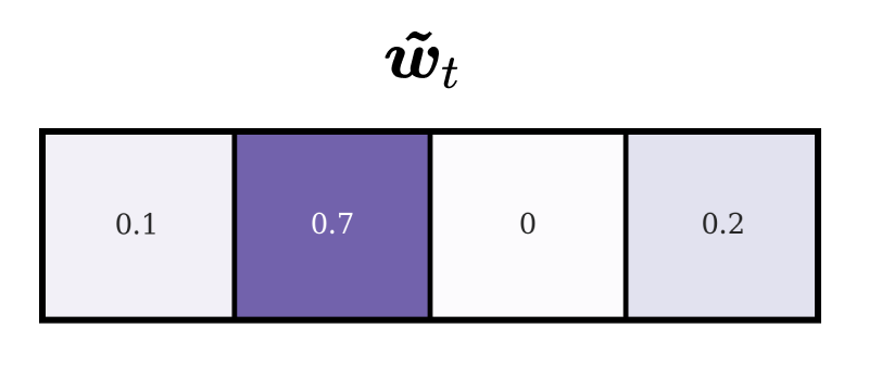
By inspecting the new attention vector we can see that the focus has been dispersed. This gives us a new insight into how our shift mechanism operates. We can observe that \(70\%\) of a given element’s value have been shifted one position forward, \(20\%\) one position backwards and \(10\%\) remain at the original position. Therefore, each dimension in \(\boldsymbol{s}_t\) specifies the amount of an element’s value that is subject to the instruction at that dimension. For example, the first dimension in \(s_t = (0.7, 0.1, 0.2)\) can be interpreted as “For each element in \(\boldsymbol{w}\), shift 70% of its original value one position forward”. The main takeaway here is that the shift weightings represent how a head’s focus should be distributed over memory locations after the shift operation and that unfocussed shift weightings lead to dispersions in the resulting attention vector.
Sharpen
To reduce the dispersions caused by the shift operation, each head receives a scalar parameter \(\gamma \geq 1\) that controls the sharpness of the weightings. The final focus vector \(\boldsymbol{w}_t\) is normalised as follows:
\[ \begin{equation} \boldsymbol{w}_{t}(i) = \frac{\tilde{\boldsymbol{w}}_{t}(i)^{\gamma_{t}}}{\sum_{j} \tilde{\boldsymbol{w}}_{t}(j)^{\gamma_{t}}} \end{equation} \]
We can visualize the effect on the memory weightings as \(\gamma\) is increased:
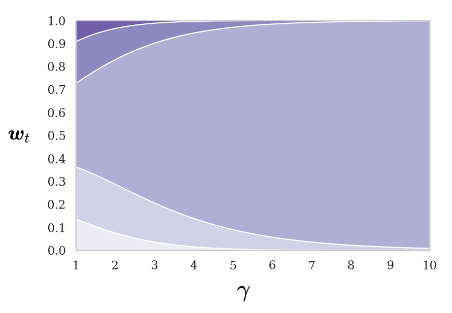
The larger \(\gamma\) is, the more focussed the final attention vector will be.
Interlude: Location-Based Addressing
Let us now build out the location-based addressing mechanism. Each step we have seen above will be implemented as a separate method. All of these will then be called successively by the focus_head method to produce the final weightings.
Gated Interpolation
Gated interpolation takes weightings from the previous time step prev_w with shape (batch_size, num_rows) and the interpolation gate g with shape (batch_size, 1) as input and blends prev_w and the content-weightings together.
class HeadBase(nn.Module):
    ...
    def focus_head(self, k, beta, g):
        w_c = self._content_weight(k, beta)
        w_g = self._gated_interpolation(w_c, prev_w, g)
        return w_g
    ...
    def _gated_interpolation(self, w, prev_w, g):
        return g*w + (1-g)*prev_w
    ...
Circular Shift
Note that for the convolutional shift we introduce a new attribute max_shift inside the constructor. This integer value indicates the maximum number of positions a head can shift at each time step. The shifted weightings are computed using the _mod_shift method. The shift weightings s are passed to the method as a tensor with shape (batch_size, 2 * max_shift + 1). As Pytorch requires 3-dimensional shapes for convolutional filters, we transform the tensor to be of shape (batch_size, 1, 2 * max_shift + 1). Next, we apply the filters to a batch of unrolled weightings. Because every filter is applied to every sequence, we obtain batch_size outputs for each input sequence i.e. output shape: (batch_size, batch_size, num_columns). We are, however, only interested in the output sequence of the \(i\)-th filter for the \(i\)-th unrolled sequence. For this reason, we need to filter the results with [range(self.batch_size), range(self.batch_size)]. The method returns a batch of shifted weightings with shape (batch_size, num_columns).
class HeadBase(nn.Module):

    def __init__(self, memory, hidden_size, max_shift):
        super(HeadBase, self).__init__()
        self.memory = memory
        self.hidden_size = hidden_size
        self.max_shift = max_shift

    def focus_head(self, k, beta, prev_w, g, s):
        w_c = self._content_weight(k, beta)
        w_g = self._gated_interpolation(w_c, prev_w, g)
        w_s = self._mod_shift(w_g, s)
        return w_g
    ...
    def _mod_shift(self, w, s):
        unrolled = torch.cat([w[:, -self.max_shift:], w, w[:, :self.max_shift]], 1)
        return F.conv1d(unrolled.unsqueeze(1),
                        s.unsqueeze(1))[range(self.batch_size), range(self.batch_size)]
    ...
Sharpen
To complete the focus_head method we implement _sharpen. In addition to the weightings, it takes the parameter gamma of shape (batch_size, 1) as input and computes the final attention vector w.
class HeadBase(nn.Module):
    ...
    def focus_head(self, k, beta, prev_w, g, s, gamma):
        w_c = self._content_weight(k, beta)
        w_g = self._gated_interpolation(w_c, prev_w, g)
        w_s = self._mod_shift(w_g, s)
        w   = self._sharpen(w_s, gamma)
        return w
    ...
    def _sharpen(self, w, gamma):
        w = w.pow(gamma)
        return torch.div(w, w.sum(1).view(-1, 1) + 1e-16)
    ...
Modes of Operation
Let’s do a quick recap and review the capabilities of the memory addressing mechanism. By combining the different operations, the network can operate in three complementary modes. First, the addressing-system can access contents purely based on the similarity with the produced key, without using location-based addressing. Second, content-based weightings can be chosen and shifted by a given number of locations. What this means in computational terms is that a head finds a block of data in memory and subsequently shifts its focus to access a particular element within that block. Third, a weighting from the previous time-step can be chosen and rotated without making use of the content-addressing mechanism. This enables the system to iterate over a sequence of memory locations by performing sequential shifts.
To sum up, we have described an addressing system that allows the network to learn how to produce attention vectors to access memory locations for read/write operations. All the mechanisms are differentiable, which makes the system trainable end-to-end.
Interlude: Heads, Controller, NTMCell
In this code interlude, we are going to finish the read and write head implementations, build a simple LSTM-based controller and create the NTMCell class that encapsulates all of our modules.
We need to implement two important functionalities. First, each head needs a way to extract the memory addressing parameters from the controller’s output. Second, we need to define the unique forward passes for both read and write heads. We implement the first point by defining a hidden_state_unpacking_scheme for each head. This method returns a list of tuples, each of which describes the length and the activation function for a given parameter. The activation functions ensure that all parameters lie within the correct numerical range. Each head is equipped with a fully-connected layer to transform the input from the controller into an internal representation, whose length is equal to the sum of the lengths of all parameters defined in the unpacking scheme. We will implement a shared method unpack_hidden_state in the HeadBase class, that allows a head to split its internal vector into a tuple of addressing parameters. Let’s now look at the individual forward passes.
Read-Head
At every time step a read head takes a batch of hidden vectors h (the controller’s instructions) with shape (batch_size, hidden_size) and the previous weightings prev_w as input. It then transforms the hidden vectors using an internal fully-connected layer fc (defined in HeadBase). Next, it uses unpack_hidden to extract the individual parameters and uses these to produce new weightings w by calling focus_head. After the head’s focus is determined, it calls the read to retrieve a read vector with shape (batch_size, num_cols) from memory. Finally, the current weightings and the read-out vectors are returned.
We initialise a head’s state using the init_state method. For a read head, it returns the initial read and attention vectors. The attention weightings are set to focus sharply on the first memory location.
class ReadHead(HeadBase):

    def __init__(self, memory, hidden_sz, max_shift):
        super(ReadHead, self).__init__(memory, hidden_sz, max_shift)

    def hidden_state_unpacking_scheme(self):
      return [
            # size, activation-function
            (self.memory.num_cols, torch.tanh),                    # k
            (1,                    F.softplus),                    # β
            (1,                    torch.sigmoid),                 # g
            (2*self.max_shift+1,   lambda x: F.softmax(x, dim=1)), # s
            (1,                    lambda x: 1 + F.softplus(x))    # γ
        ]

    def read(self, w):
        return torch.matmul(w.unsqueeze(1), self.memory.data).squeeze(1)

    def forward(self, h, prev_w):
        k, beta, g, s, gamma = self.unpack_hidden_state(self.fc(h))
        w = self.focus_head(k, beta, prev_w, g, s, gamma)
        read = self.read(w)
        return read, w

    def init_state(self, batch_size, device):
        self.batch_size = batch_size
        reads      = torch.zeros(batch_size, self.memory.num_cols).to(device)
        read_focus = torch.zeros(batch_size, self.memory.num_rows).to(device)
        read_focus[:, 0] = 1.
        return reads, read_focus
Write-Head
The write head follows the same principle but its unpacking scheme now also includes the erase vector e and add vector a, both of shape (batch_size, num_cols). After extracting the parameters, the head calls the write method to update the previous memory. Finally, the head returns the weightings used for the writing operation.
For write heads, the init_state method only returns the head’s initial attention vectors. Again, each of these is set to focus sharply on the first memory location.
class WriteHead(HeadBase):

    def __init__(self, memory, hidden_sz, max_shift):
        super(WriteHead, self).__init__(memory, hidden_size, max_shift)

    def hidden_state_unpacking_scheme(self):
        return [
            # size, activation-function
            (self.memory.num_cols, torch.tanh),                    # k
            (1,                    F.softplus),                    # β
            (1,                    torch.sigmoid),                 # g
            (2*self.max_shift+1,   lambda x: F.softmax(x, dim=1)), # s
            (1,                    lambda x: F.softplus(x) + 1),   # γ
            (self.memory.num_cols, torch.sigmoid),                 # e
            (self.memory.num_cols, torch.tanh)                     # a
        ]

    def erase(self, w, e):
        return self.memory.data * (1 - w.unsqueeze(2) * e.unsqueeze(1))

    def write(self, w, e, a):
        memory_erased    = self.erase(w, e)
        self.memory.data = memory_erased + (w.unsqueeze(2) * a.unsqueeze(1))

    def forward(self, h, prev_w):
        k, beta, g, s, gamma, e, a = self.unpack_hidden_state(self.fc(h))

        w = self.focus_head(k, beta, prev_w, g, s, gamma)
        self.write(w, e, a)

        return w

    def init_state(self, batch_size, device):
        self.batch_size = batch_size
        write_focus = torch.zeros(batch_size, self.memory.num_rows).to(device)
        write_focus[:, 0] = 1.
        return write_focus
Head-Base
Here we show the final implementation of the HeadBase class. Take a look at the unpack_hidden_state method to see how the individual parameters are extracted from the hidden vector and how the appropriate activation functions are applied.
class HeadBase(nn.Module):

    def __init__(self, memory, hidden_size, max_shift):
        super(HeadBase, self).__init__()

        self.memory = memory
        self.hidden_size = hidden_size
        self.max_shift = max_shift

        self.fc = nn.Linear(hidden_size,
                            sum([s for s, _ in self.hidden_state_unpacking_scheme()]))

        self.init_params()

    def forward(self, h):
        raise NotImplementedError

    def hidden_state_unpacking_scheme():
        raise NotImplementedError

    def unpack_hidden_state(self, h):
        chunk_idxs, activations = zip(*self.hidden_state_unpacking_scheme())
        chunks = torch.split(h, chunk_idxs, dim=1)
        return tuple(activation(chunk) for chunk, activation in zip(chunks, activations))

    def focus_head(self, k, beta, prev_w, g, s, gamma):
        w_c = self._content_weight(k, beta)
        w_g = self._gated_interpolation(w_c, prev_w, g)
        w_s = self._mod_shift(w_g, s)
        w = self._sharpen(w_s, gamma)
        return w

    def _content_weight(self, k, beta):
        k = k.unsqueeze(1).expand_as(self.memory.data)
        similarity_scores = F.cosine_similarity(k, self.memory.data, dim=2)
        w = F.softmax(beta * similarity_scores, dim=1)
        return w

    def _gated_interpolation(self, w, prev_w, g):
        return g*w + (1-g)*prev_w

    def _mod_shift(self, w, s):
        unrolled = torch.cat([w[:, -self.max_shift:], w, w[:, :self.max_shift]], 1)
        return F.conv1d(unrolled.unsqueeze(1),
                        s.unsqueeze(1))[range(self.batch_size), range(self.batch_size)]

    def _sharpen(self, w, gamma):
        w = w.pow(gamma)
        return torch.div(w, w.sum(1).view(-1, 1) + 1e-16)

    def init_state(self, batch_size):
        raise NotImplementedError

    def init_params(self):
        pass
Controller
The controller could be either a recurrent or a fully-connected neural network. As an example, I use a simple recurrent controller based on stacked LSTM-cells. The controller takes the concatenation of the current inputs xb and the previous read-vectors prev_reads as input (see implementation of NTMCell) and returns a hidden state h of shape (batch_size, hidden_size). This hidden state is used to parametrise the heads. Moreover, it returns a list of tuples hidden_states containing the hidden and cell states of each recurrent layer.
The method init_state returns the intial hidden and cell states for the stacked-LSTM.
class LSTMCellController(nn.Module):
    def __init__(self, input_size, hidden_size, num_layers):
        super().__init__()
        self.input_size = input_size
        self.hidden_size = hidden_size

        self.fc = nn.Linear(input_size, hidden_size)
        self.cells = nn.ModuleList(
            [nn.LSTMCell(hidden_size, hidden_size) for _ in range(num_layers)]
        )

        self.init_params()

    def forward(self, xb, prev_hidden_states):

        hidden_states = []
        h = self.fc(xb)

        for i, cell in enumerate(self.cells):
            h, c = cell(h, prev_hidden_states[i])
            hidden_states += [(h, c)]

        return h, hidden_states

    def init_state(self, batch_size, device):
        h = torch.zeros(self.num_layers, self.batch_size, self.hidden_size).to(device)
        c = torch.zeros(self.num_layers, self.batch_size, self.hidden_size).to(device)
        return list(zip(h, c))

    def init_params(self):
        pass
Neural Turing Machine Cell
Finally, we can finish our implementation by defining the NTMCell class, which will encapsulate all the modules we have created so far. Besides computing the output, its main function is to instantiate the memory, the heads and the controller. The NTM’s state is represented as a named tuple and includes the read vectors returned by the read heads, the focus weights used by both the read and write heads and the hidden and cell states of the LSTM-controller. Let us now take a look at the forward method. At each time step, the NTM-cell receives inputs xb with shape (batch_size, input_size). If no input is specified, the NTM will receive a batch of zero vectors. The first step is to unpack the previous state. Next, we concatenate the previous read vectors prev_reads with the current input xb. These sequences are then passed to the controller, which returns its hidden state (the parameters for the heads) and a list of tuples storing the hidden and cell state of each layer. In the second step, we iterate over the list of heads and each head executes a read or write operation. Attention weightings for read and write heads as well as read vectors are collected in separate lists. These lists, together with the controller’s hidden and cell states, are then stored in a new state tuple. In a final step, the hidden state returned by the controller is concatenated with the current read-out vectors and passed through a fully-connected layer to create the final output.
Have a look at the init_state method, to see how the NTM initialises the states of its submodules.
class NTMCell(nn.Module):

    def __init__(self,
                 input_size,
                 hidden_size,
                 output_size,
                 memory_num_rows,
                 memory_num_cols,
                 controller_num_layers=3,
                 num_heads=1,
                 max_shift=1):

        super().__init__()

        self.input_size = input_size
        self.hidden_size = hidden_size
        self.output_size = output_size

        self.num_heads = num_heads
        self.max_shift = max_shift

        self.memory_num_rows = memory_num_rows
        self.memory_num_cols = memory_num_cols

        self.state_container = namedtuple('state', [
            'read_vectors', 'read_focus_weights', 'write_focus_weights', 'hidden_states'
        ])

        self.batch_size = None

        # module instantiations
        self.memory = Memory(memory_num_rows, memory_num_cols)


        self.controller_num_layers = controller_num_layers
        self.controller = LSTMCellController(input_size + num_heads * memory_num_cols, hidden_size, controller_num_layers)

        # create heads
        self.read_heads = nn.ModuleList([
            ReadHead(self.memory, hidden_size, max_shift)
            for _ in range(num_heads)
        ])
        self.write_heads = nn.ModuleList([
            WriteHead(self.memory, hidden_size, max_shift)
            for _ in range(num_heads)
        ])

        self.fc = nn.Linear(hidden_size + num_heads * memory_num_cols, output_size)

        self.init_params()

    def forward(self, xb=None):
        if xb is None:
            xb = torch.zeros(self.batch_size, self.input_size).to(self.device)

        # unpacking the previous state
        prev_reads      = self.state.read_vectors
        prev_hiddens    = self.state.hidden_states
        prev_read_foci  = self.state.read_focus_weights
        prev_write_foci = self.state.write_focus_weights

        xb = torch.cat([xb, *prev_reads], dim=1)

        # controller output
        h, hidden_states  = self.controller(xb, prev_hiddens)

        # read and write
        reads      = []
        read_foci  = []
        write_foci = []

        for i, (read_head, write_head) in enumerate(zip(self.read_heads, self.write_heads)):
            read, read_focus = read_head(h,  prev_read_foci[i])    # read
            write_focus      = write_head(h, prev_write_foci[i])   # write

            reads      += [read]
            read_foci  += [read_focus]
            write_foci += [write_focus]

        # pack new state
        self.state = self.state_container(reads, read_foci, write_foci, hidden_states)

        # output
        out = torch.cat([h, *reads], dim=1)
        return self.fc(out)

    def init_params(self):
        pass

    def init_state(self, batch_size, device):
        self.batch_size = batch_size
        self.device = device

        # Initialize the memory
        self.memory.init_state(batch_size, device)

        # hidden state init
        hidden_states = self.controller.init_state(batch_size, device)

        # init heads and collect initial read vectors, read foci and write foci
        reads      = []
        read_foci  = []
        write_foci = []

        for rh, wh in zip(self.read_heads, self.write_heads):
            read, read_focus = rh.init_state(batch_size, device)
            write_focus      = wh.init_state(batch_size, device)

            reads      += [read]
            read_foci  += [read_focus]
            write_foci += [write_focus]

        # pack the initial state
        self.state = self.state_container(reads, read_foci, write_foci, hidden_states)
That’s the entire architecture! Before you can use the NTM, however, you will have to initialise the network’s weights. Every module containing learnable parameters has a method init_params that is called when the module is instantiated. You can use this to experiment with different parameter initialisations in a modular way.
Finally, the NTMCell can be initialised and reset in the following way:
ntm = NTMCell(input_size,
              hidden_size,
              output_size,
              memory_num_rows,
              memory_num_cols,
              controller_num_layers,
              num_heads,
              max_shift)

ntm = ntm.to(device)
ntm.init_state(batch_size, device) # init state of all modules

...

# reset within training loop
ntm.init_state(batch_size, device)
Some Shortcomings
The main shortcoming of the Neural Turing Machine and arguably the one that prevents mainstream adoption is that the architecture is notoriously difficult to train. Even though the writing mechanism makes the architecture more powerful than read-only systems, learning how to write information to and read back from memory creates an extremely difficult coupled learning problem (Graves 2018). In the next section, we will look at some tricks that can help to mitigate numerical instabilities.
Another problem is that temporal information is neglected. Think about how hearing a specific song or smelling a particular smell takes you back to a related moment in the past. This association is not an isolated memory. We usually also remember a kind of temporal window around the retrieved moment (Graves 2018). Even though, our shift mechanism can move a head’s focus to adjacent memory locations, this does not automatically imply that there exists a temporal link between the memories.
The Differentiable Neural Computer (Graves et al. 2016) is an architecture that tries to resolve some of these shortcomings. Among other improvements, it replaces the shift mechanism with a temporal link matrix and extends the NTM by a differentiable free list to allocate and deallocate memory.
Interlude: NTM Training Tricks
In this last code interlude, I will list some tricks that can help to make the training of the NTM numerically stable. Many of these were adopted from a paper by Collier et. al.(Collier and Beel 2018), as well as existing open source implementations.
Initialisations
Initial Hidden and Cell State
In my experience, learning the initial values of the hidden and cell state, the initial read vector and the initial focus of read/write-heads often helped to stabilise the training process.
To learn the initial hidden and cell states of an LSTM controller, we add two new tensors h_bias and c_bias to our constructor. These tensors hold trainable parameters that are updated during training. When the NTM is instantiated or reset, init_state is called. The bias tensors are extended to entire batches and moved to the appropriate device. Additionally, it can be helpful to scale-down the initial random biases using a small value alpha e.g. 0.05.
class LSTMCellController(nn.Module):
    def __init__(self, input_size, hidden_size, num_layers):
        ...
        self.h_bias = nn.Parameter(torch.rand(self.num_layers, 1, self.hidden_size) * alpha)
        self.c_bias = nn.Parameter(torch.rand(self.num_layers, 1, self.hidden_size) * alpha)
        ...

    def init_state(self, batch_size, device):
        h = self.h_bias.clone().repeat(1, batch_size, 1).to(device)
        c = self.c_bias.clone().repeat(1, batch_size, 1).to(device)
        return list(zip(h, c))
Initial Read Vector, Read Attention and Write Attention
We can follow the same approach to learn the initialisation of read and focus vectors. The only difference is that we need to apply the softmax activation function to the attention vectors as these need to be normalised.
class ReadHead(HeadBase):

    def __init__(self, memory, hidden_size, max_shift):
        super(ReadHead, self).__init__(memory, hidden_sz, max_shift)

        self.read_bias       = nn.Parameter(torch.randn(1, self.memory.num_cols))
        self.read_focus_bias = nn.Parameter(torch.randn(1, self.memory.num_rows))

    ...

    def init_state(self, batch_size, device):
        self.batch_size = batch_size
        reads      = self.read_bias.clone().repeat(batch_size, 1).to(device)
        read_focus = self.read_focus_bias.clone().repeat(batch_size, 1).to(device)
        return reads, torch.softmax(read_focus, dim=1)
And again for the initial attention vector for the write heads…
class WriteHead(HeadBase):

    def __init__(self, memory, hidden_size, max_shift):
        super(WriteHead, self).__init__(memory, hidden_sz, max_shift)
        self.write_focus_bias = nn.Parameter(torch.rand(1, self.memory.num_rows))

    ...

    def init_state(self, batch_size, device):
        self.batch_size = batch_size
        write_focus = self.write_focus_bias.clone().repeat(batch_size, 1).to(device)
        return torch.softmax(write_focus, dim=1)
Initial Memory
For the memory state, we deviate from our learned initialisation strategy. Collier et. al. (Collier and Beel 2018) showed that on a subset of the original algorithmic tasks the best approach was to initialise the memory contents with a small constant value e.g. \(10^{-6}\). If the memory matrix is large, constant initialisation reduces the number of trainable parameters substantially.
class Memory(nn.Module):

    def __init__(self, num_rows, num_cols):
        super(Memory, self).__init__()

        self.num_rows = num_rows
        self.num_cols = num_cols

        self.mem_bias = torch.Tensor().new_full((num_rows, num_cols), 1e-6)

    def init_state(self, batch_size, device):
        self.data = self.mem_bias.clone().repeat(batch_size, 1, 1).to(device)
Forget-Gate Bias and Gradient Clipping
Two more tricks we can use to make the training process more stable is to clip the gradients and initialise the bias of the forget-gate to a positive value \(\geq 1\). Using larger positive values for the bias pushes the forget-gate’s sigmoid activation very close to one. This has the effect that at the beginning of the training phase the model degenerates into a standard LSTM. It will not explicitly forget anything until it has learned to forget (Gers, Schmidhuber, and Cummins 1999). Although Pytorch does not have an explicit way to set the bias of the forget-gate, we can create our own function by exploiting the fact that the bias vector of an LSTMCell (or LSTM) layer has the structure [bias_ig | bias_fg | bias_gg | bias_og].
def set_forget_gate_(tensor, val=1.0):
    """
    Initialise the biases of the forget gate to `val`, and all other gates to 0.
    """
    # gates are (b_hi|b_hf|b_hg|b_ho) of shape (4*hidden_size)
    tensor.data.zero_()
    hidden_size = tensor.shape[0] // 4
    tensor.data[hidden_size:(2 * hidden_size)] = val
We can use this function within our LSTM’s init_params method to set the bias value.
class LSTMCellController(nn.Module):
    def __init__(self, input_size, hidden_size, num_layers):
        super().__init__()
        ...
        self.cells = nn.ModuleList(
            [nn.LSTMCell(hidden_size, hidden_size) for _ in range(num_layers)]
        )
        ...
        self.init_params()

    ...

    def init_params(self):
        ...
        for param in self.cells.parameters():
            if param.dim() < 2:
                set_forget_gate_(param, 1.0)
            else:
              ...
Both reference papers (Graves, Wayne, and Danihelka 2014; Collier and Beel 2018) employed gradient clipping to prevent spikes in the gradients. In Pytorch gradient clipping can be implemented inside the training loop using the clip_grad_norm_ function:
loss.backward()
clip_grad_norm_(model.parameters(), max_norm)
optimizer.step()
optimizer.zero_grad()
What’s Next?
In this post, we have learned about the Neural Turing Machine, a differentiable computer, that can learn simple programs using inputs from its environment. We covered both the mathematical definitions and implemented the architecture from scratch using the Pytorch library. I hope you leave with an intuitive understanding of the main architectural components and memory access mechanisms. As I get deeper into the literature, I will cover more architectures, both historical and contemporary. Moreover, I want to complement my usual readings in artificial intelligence and machine learning with more related research from neuroscience. Finally, I am planning to experiment with memory-enhanced agents in different reinforcement learning settings, with the goal of discovering useful memory priors.
If you have questions or find errors please reach out on Twitter or send an email to schmidinger.n AT gmail.com.
Collier, Mark, and Joeran Beel. 2018. “Implementing Neural Turing Machines.” Lecture Notes in Computer Science, 94–104. https://doi.org/10.1007/978-3-030-01424-7_10.
Gers, Felix A, Jürgen Schmidhuber, and Fred Cummins. 1999. “Learning to Forget: Continual Prediction with Lstm.”
Graves, Alex. 2018. “Advanced Deep Learning & Reinforcement Learning Lecture 17: Attention and Memory in Deep Learning.” YouTube. DeepMind. https://www.youtube.com/watch?v=Q57rzaHHO0k&list=PLqYmG7hTraZDNJre23vqCGIVpfZ_K2RZs&index=15.
Graves, Alex, Greg Wayne, and Ivo Danihelka. 2014. “Neural Turing Machines.” https://arxiv.org/abs/1410.5401.
Graves, Alex, Greg Wayne, Malcolm Reynolds, Tim Harley, Ivo Danihelka, Agnieszka Grabska-Barwińska, Sergio Gómez Colmenarejo, et al. 2016. “Hybrid Computing Using a Neural Network with Dynamic External Memory.” Nature 538 (7626): 471.
Ha, Junsoo. 2017. “Neural Turing Machines Pytorch Implementation.” GitHub Repository. GitHub. https://github.com/kuc2477/pytorch-ntm.
Zana, Guy. 2017. “PyTorch Neural Turing Machine (Ntm).” GitHub Repository. GitHub. https://github.com/loudinthecloud/pytorch-ntm.
The way how the heads are parameterised by the outputs of the controller is an important lesson for developing neural architectures. First, come up with a functional form for a desired mechanism and then let another network generate parameters for the given function.↩︎
Note that I chose binary vectors for my examples because intermediate values are easy to calculate in one’s mind and patterns of calculations become more apparent visually. In practice, however, the memory will usually hold real-valued vectors.↩︎
Note that to fully erase a cell, a head needs to sharply focus on a single memory location and the corresponding element of \(\boldsymbol{e}\) needs to be \(1\).↩︎