Table of Contents
Introduction
Figure 1: The sorcerer’s apprentice. Illustration by Ferdinand Barth circa 1882.
Gone’s for once the old magician
With his countenance forbidding;
I ’m now master,
I ’m tactician,
All his ghosts must do my bidding.
Know his incantation,
Spell and gestures too;
By my mind’s creation
Wonders shall I do.
– Johann Wolfgang von Goethe (The sorcerer’s apprentice)
While mulling over old papers and hacking away at their computers, scholars build up an intimate knowledge about their research topic. As they chart their way through idea space, they develop a deep intuition on which techniques work well in practice. Unfortunately, many of these hard-earned insights are not published and remain obscure.
Last year, I took a course at the Johannes Kepler University in Linz, Austria on the topic of Recurrent Neural Networks and Long Short-Term Memory Networks. There, Sepp Hochreiter shared some of the “magic tricks” he and his team employ for training LSTMs. This blog post is the accumulation of some of my notes.
For this post, I assume you are already familiar with LSTMs. If not, I suggest you begin with Chris Olah’s Understanding LSTM Networks and then go on to read the original LSTM work (Hochreiter and Schmidhuber 1997).
Before we begin, I’d also like to highlight some resources that are similar in their motivation:
- Andrej Karpathy’s general recipe for training neural networks.
- Danijar Hafner’s tips for training recurrent neural networks (Hafner 2017).
- LSTM: A Search Space Odyssey (Greff et al. 2017) from IDSIA (Dalle Molle Institute for Artificial Intelligence).
In case you want to experiment with some of the presented techniques and you need a flexible Pytorch-based LSTM implementation, I recommend Michael Widrich’s LSTM Tools library.
All credits for the presented techniques go to the authors. All errors in their presentation are mine. I am always keen to receive feedback.
Vanilla LSTM
The Vanilla LSTM is one of the most prevalent variants and is often the default LSTM architecture in popular software libraries. It is characterized by three gates and a memory state – the gates provide the model with capacity and protect the memory cells from distracting information and noise; they make the dynamics of the LSTM highly non-linear and allow it to learn to perform complex operations.
Let us briefly step through the Vanilla LSTM’s mechanics to introduce the notation and terminology used in this post. Sensory inputs \(\boldsymbol{x}(t)\) flowing into the LSTM cell at a given time step are transformed into the cell input activation \(\boldsymbol{z}(t)\) – the elements of \(\boldsymbol{z}(t)\) are activated by a non-linear function \(g(\cdot)\), which in practice is often defined as the hyperbolic tangent or tanh. Information that is irrelevant for the current time step is removed by multiplying \(\boldsymbol{z}(t)\) element-wise by a sigmoid-activated input gate \(\boldsymbol{i}(t)\). Similarily, the cell state of the previous time step \(\boldsymbol{c}(t-1)\) is partially erased using a sigmoid-activated forget gate \(\boldsymbol{f}(t)\). The new memory cell state \(\boldsymbol{c}(t)\) is computed by adding the current cell state update \(\boldsymbol{i}(t) \odot \boldsymbol{z}(t)\) to the the filtered old state \(\boldsymbol{f}(t) \odot \boldsymbol{c}(t-1)\). Finally, the LSTM squashes the memory contents into a specific numerical range using the memory cell activation function \(h(\cdot)\) and filters the result through an output gate \(\boldsymbol{o}(t)\). This results in the final memory cell state activation \(\boldsymbol{y}(t)\).
Mathematically, the Vanilla LSTM can be defined by the following set of equations:
\[ \begin{align} \boldsymbol{i}(t) &= \sigma\left(\boldsymbol{W}_{i}^{\top} \boldsymbol{x}(t)+\boldsymbol{R}_{i}^{\top} \boldsymbol{y}(t-1)\right) \\ \boldsymbol{o}(t) &= \sigma\left(\boldsymbol{W}_{o}^{\top} \boldsymbol{x}(t)+\boldsymbol{R}_{o}^{\top} \boldsymbol{y}(t-1)\right) \\ \boldsymbol{f}(t) &= \sigma\left(\boldsymbol{W}_{f}^{\top} \boldsymbol{x}(t)+\boldsymbol{R}_{f}^{\top} \boldsymbol{y}(t-1)\right) \\ \boldsymbol{z}(t) &= g\left(\boldsymbol{W}_{z}^{\top} \boldsymbol{x}(t)+\boldsymbol{R}_{z}^{\top} \boldsymbol{y}(t-1)\right) \\ \boldsymbol{c}(t) &= \boldsymbol{f}(t) \odot \boldsymbol{c}(t-1)+\boldsymbol{i}(t) \odot \boldsymbol{z}(t) \\ \boldsymbol{y}(t) &= \boldsymbol{o}(t) \odot h(\boldsymbol{c}(t)) \end{align} \]
Where \(\sigma\) denotes the sigmoid activation function and \(\odot\) the element-wise or Hadamard product. Note that each of the gates has access to the current input \(\boldsymbol{x}(t)\) and the previous cell state activation \(\boldsymbol{y}(t-1)\).
Also remember, that the weights \(W\) and recurrent weights \(R\) are shared between time steps.
![Schematic of the Vanilla LSTM Cell with unrolled cell state. Figure adopted from [@Greff_2017].](images/vanilla_lstm_legend.png)
Figure 2: Schematic of the Vanilla LSTM Cell with unrolled cell state. Figure adopted from (Greff et al. 2017).
Input Activation Functions and the Drift Effect
In practice, the input activation function \(g\) is often chosen to be tanh. But this choice is non-obvious and in fact, in the original LSTM paper sigmoid was used to activate \(\boldsymbol{z}\). As the memory cell’s purpose is to learn and memorise patterns over time, sigmoid activations are a natural choice to indicate the presence (activation with a value close to \(1\)) or absence (activation with a value close to \(0\)) of entities in the input. Tanh on the other hand with a lower bound of \(-1\) doesn’t seem to make intuitive sense. What is a negative pattern? Does an activation with value \(-1\) indicate that something is strongly not present in the input?
The adoption of tanh first required two mental shifts. First, tanh makes intuitive sense in a meta-learning setting. Instead of patterns, we now use memory cells to store the weights for another neural network. To indicate whether the values of the weights should be increased or decreased we need both positive and negative values.
The second intuitive interpretation is the storage of hints. A hint in this context is evidence in favour of or against something. Consider an example from text analysis. Assume that a model encounters the words “Team”, “Player” and “Goal” in a paragraph. These are all strong hints that the text is about sports, but if the next passage includes the words “Manager”, “Revenue” and “Shareholder” it is a strong indication that the paragraph actually describes a business context. Positive values can be seen as hints in favour of and negative values as hints against certain classes.
But there is a simple mathematical reason why tanh is the preferred choice to activate the cell input. Compared to commonly used activation functions such as ReLU and sigmoid the expected value of the cell input activation is zero for tanh (under the assumption of zero-mean Gaussian pre-activations):
\[\mathbb{E}(\boldsymbol{z}(t)) = 0\]
To understand why this property is desirable, remember how the cell state is updated at a given time step1:
\[\boldsymbol{c}(t) = \boldsymbol{c}(t-1)\color{#9900ff}{+\boldsymbol{i}(t) \odot \boldsymbol{z}(t)}\]
At each time step we add the cell input activation \(\boldsymbol{z}(t)\) (filtered by the input gate) to the previous cell state \(\boldsymbol{c}(t-1)\). If we choose an activation function for \(\boldsymbol{z}\), such that each activation has a value \(\geq 0\) (e.g. sigmoid, ReLU, etc.), \(\boldsymbol{c}\) will quickly take on very large values. Even if the activations are relatively small, the cell state will grow large for sufficiently long sequences. This problem is known as the drift effect.
But how can large memory cell states become a hindrance to learning? To answer this question, we need to take a look at the LSTM’s backward pass:
\[ \begin{aligned} \frac{\partial L}{\partial \boldsymbol{c}(t)} &=\frac{\partial L}{\partial \boldsymbol{y}(t)} \color{#9900ff}{\frac{\partial \boldsymbol{y}(t)}{\partial \boldsymbol{c}(t)}}+\frac{\partial L}{\partial \boldsymbol{c}(t+1)} \frac{\partial \boldsymbol{c}(t+1)}{\partial \boldsymbol{c}(t)} \\ &=\frac{\partial L}{\partial \boldsymbol{y}(t)} \operatorname{diag}\left(\boldsymbol{o}(t) \odot \color{#9900ff}{h^{\prime}(\boldsymbol{c}(t))}\right)+\frac{\partial L}{\partial \boldsymbol{c}(t+1)} \end{aligned} \]
The equation recursively sums up all error signals from the future and carries them backwards in time. Intuitively, it describes the different ways in which the cell state at time \(t\) influences the loss \(L\). We take a closer look at the highlighted term \(\partial \boldsymbol{y}(t) / \partial \boldsymbol{c}(t)\) , which describes how the memory cell state activation \(\boldsymbol{y}(t)\) changes as \(\boldsymbol{c}(t)\) changes. The partial derivative can be obtained by calculating \(\operatorname{diag}\left(\boldsymbol{o}(t) \odot h^{\prime}(\boldsymbol{c}(t))\right)\). And now we are in trouble. Remember that we use the tanh as the memory cell activation function \(h\) to squash the memory cell state into the numerical range \((-1, 1)\). Its derivative is defined as follows:
\[ h^{\prime}(\boldsymbol{x}) = \text{tanh}^{\prime}(\boldsymbol{\boldsymbol{x}}) = 1 - \text{tanh}²(\boldsymbol{x}) \]
Now if \(\boldsymbol{c}(t)\) grows very large due to the drift effect, the highlighted term in the second equation will evaluate to \(h^{\prime}(\boldsymbol{c}(t)) = 1-1 = 0\) for each element in \(\boldsymbol{c}(t)\). As a result, \(\frac{\partial L}{\partial y(t)} \frac{\partial y(t)}{\partial c(t)}\) will be zero and the cell state loses its ability to influence the memory cell state activation \(\boldsymbol{y}(t)\) and as a result the loss \(L\).
We can see that choosing tanh as our input activation function \(g\) is superior to other commonly used functions because it eliminates the drift effect. With its range centred around zero, the cell state is prevented from accumulating over time. This in turn stabilises the learning signal, which is key to learning long-term dependencies.
Forget Gates and Vanishing Gradients
To prevent the cell state from accumulating, Felix Gehrs and Jürgen Schmidhuber proposed the forget gate (Gers, Schmidhuber, and Cummins 1999). The idea is to allow the network to learn to erase the cell state before each update.
\[ \begin{array}{l} f(t)=\sigma\left(W_{f}^{\top} x(t)+R_{f}^{\top} y(t-1)\right) \\ c(t)=\color{#9900ff}{f(t) \odot c(t-1)}+i(t) \odot z(t) \end{array} \]
The main problem of the forget gate, however, is that it can reintroduce the vanishing gradient problem — which, paradoxically, the LSTM architecture was built to eliminate in the first place. Let’s take a look at how the forget gate influences the gradients:
\[ \frac{\partial L}{\partial \boldsymbol{c}(t)}=\frac{\partial L}{\partial \boldsymbol{y}(t)} \frac{\partial \boldsymbol{y}(t)}{\boldsymbol{c}(t)}+\frac{\partial L}{\partial \boldsymbol{c}(t+1)} \color{#9900ff}{\frac{\partial \boldsymbol{c}(t+1)}{\partial \boldsymbol{c}(t)}} \]
Without a forget gate, the gradient is equal to the identity matrix. The vanishing gradient problem is eliminated:
\[ \frac{\partial \boldsymbol{c}(t+1)}{\partial \boldsymbol{c}(t)}=\boldsymbol{I}_{I} \]
With a forget gate, on the other hand, the gradient becomes:
\[ \frac{\partial \boldsymbol{c}(t+1)}{\partial \boldsymbol{c}(t)}=\operatorname{diag}(\boldsymbol{f}(t+1)) \]
The resulting matrix is generally no longer norm-preserving.
Even though its use may be controversial, the forget gate typically works very well in situations when training sequences are short. To reduce the impact of problematic gradients it is advisable to initialise the bias units of the forget gate with large positive values. This biases the gate to be open initially (activations close to one) and pushes the gradient towards the identity matrix.
A common variation of the forget gate is to tie it to the input gate. Old information is erased from the cell state to the same degree as to which new information is allowed to flow in. The result is a simplified architecture with less trainable parameters2. The cell state is updated as follows:
\[ \boldsymbol{c}(t)=(\mathbf{1}-\boldsymbol{i}(t)) \odot \boldsymbol{c}(t-1)+\boldsymbol{i}(t) \odot \boldsymbol{z}(t) \]
Focused LSTM
The Focused LSTM is a simplified LSTM variant with no forget gate. Its main motivation is a separation of concerns between the cell input activation \(\boldsymbol{z}(t)\) and the gates. In the Vanilla LSTM both \(\boldsymbol{z}\) and the gates depend on the current external input \(\boldsymbol{x}(t)\) and the previous memory cell state activation \(\boldsymbol{y}(t-1)\). This can lead to redundancies between \(\boldsymbol{i}\) and \(\boldsymbol{z}\). For \(\boldsymbol{i}(t) \odot \boldsymbol{z}(t)\) to be activated both \(\boldsymbol{i}\) and \(\boldsymbol{z}\) need to be active and because both access the same information, they typically learn similar weights (i.e. they detect the same patterns) or either one of them converges to a constant value3.
With Focused LSTMs, \(\boldsymbol{z}\) only sees the current input \(\boldsymbol{x}(t)\) and the gates base their decisions solely on the previous memory cell state activation \(\boldsymbol{y}(t-1)\). First, \(\boldsymbol{z}\) detects patterns in the input sequence, and the input gate then scales \(\boldsymbol{z}\) based on the internal state.
\[ \begin{array}{l} {\boldsymbol{i}(t)=\sigma\left(\boldsymbol{R}_{i}^{\top} \boldsymbol{y}(t-1)\right)} \\ {\boldsymbol{o}(t)=\sigma\left(\boldsymbol{R}_{o}^{\top} \boldsymbol{y}(t-1)\right)} \\ {\boldsymbol{z}(t)=g\left(\boldsymbol{W}^{\top} \boldsymbol{x}(t)\right)} \\ {\boldsymbol{c}(t)=\boldsymbol{c}(t-1)+\boldsymbol{i}(t) \odot \boldsymbol{z}(t)} \\ {\boldsymbol{y}(t)=\boldsymbol{o}(t) \odot h(\boldsymbol{c}(t))} \end{array} \]
This division of information access has some advantages over the Vanilla LSTM. First, the number of trainable parameters is reduced to \(2 I^{2}+I D\) without bias units — where \(D\) and \(I\) are the input and hidden dimensions respectively. Second, the only way for new information to enter the memory cell is now via \(\boldsymbol{z}\). This makes it much easier to analyse and reason about the dynamics of the LSTM and, hence, can aid explainability.
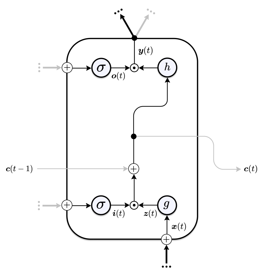
Figure 3: Schematic of the Focused LSTM Cell.
Lightweight LSTM
We continue dismantling the Vanilla LSTM’s machinery. By removing the output gate from the Focused LSTM we arrive at the Lightweight LSTM architecture:
\[ \begin{array}{l} {\boldsymbol{i}(t)=\sigma\left(\boldsymbol{R}_{i}^{\top} \boldsymbol{y}(t-1)\right)} \\ {\boldsymbol{z}(t)=g\left(\boldsymbol{W}^{\top} \boldsymbol{x}(t)\right)} \\ {\boldsymbol{c}(t)=\boldsymbol{c}(t-1)+\boldsymbol{i}(t) \odot \boldsymbol{z}(t)} \\ {\boldsymbol{y}(t)=h(\boldsymbol{c}(t))} \end{array} \]
Why would we want to do that? Again, we trade degrees of freedom of the network for a smaller number of parameters, increased speed and interpretability. Another reason is redundancy. In the Vanilla/Focused LSTM, information is first filtered by the output gate of the current cell and is then piped into the input gate of the next cell. We can simplify this two-step process by giving the input gate access to the unfiltered information and discarding the output gate. Another possible drawback of the output gate is that it can lead to oscillations—the output gate opens and closes at alternating time steps4.
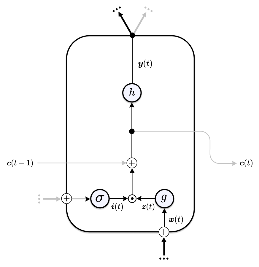
Figure 4: Schematic of the Lightweight LSTM Cell.
Ticker Steps
Imagine reading a book. We don’t read linearly. We jump back and forth and occasionally pause and ponder after reading a difficult passage. Recurrent Networks cannot do this. They don’t have an internal mechanism that allows them to pause and mull over, for example, a certain token in a sequence. An RNN spends an equal amount of computation at every time step.
A simple way to mimic pondering algorithmically is to repeatedly feed the previous input or a neutral element (e.g. zero tensors) to the network at a given time step – We let the input ticker for a certain number of times. The intuition behind these additional ticker or ponder steps is to increase the level of abstraction of the network. A recurrent neural network can be viewed as a feed-forward neural network where the number of layers is the same as the length of the input sequences and weights are shared between layers. By repeating certain elements we can create deeper and more expressive networks with a depth beyond that which is naturally defined by the input sequences.
This notion, however, introduces some problems. Should the network emit outputs at these ponder steps? How many steps should we let the input ticker? Which time steps should be repeated?
These problems are addressed by the Adaptive Computation Time algorithm by Alex Graves (Graves 2016). The presented mechanism allows an RNN to learn how many ponder steps to take between receiving an input and emitting an output:
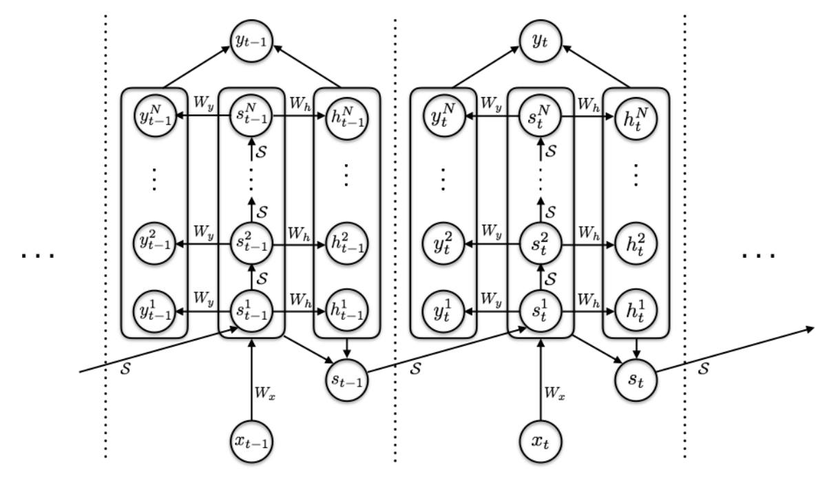
Figure 5: RNN Computation Graph with Adaptive Computation Time. Source: arxiv.org/abs/1603.08983
At every time step, the RNN computes a sequence of intermediate states \(\left(s_{t}^{1}, \ldots, s_{t}^{N(t)}\right)\) and a sequence of intermediate outputs \(\left(y_{t}^{1}, \ldots, y_{t}^{N(t)}\right)\) using the following set of equations:
\[ \begin{array}{l} s_{t}^{n}=\left\{\begin{array}{l} \mathcal{S}\left(s_{t-1}, x_{t}^{1}\right) \text { if } n=1 \\ \mathcal{S}\left(s_{t}^{n-1}, x_{t}^{n}\right) \text { otherwise } \end{array}\right. \\ y_{t}^{n}=W_{y} s_{t}^{n}+b_{y} \end{array} \]
where \(\mathcal{S}\) is the state-transition function (for example an LSTM cell).
But how does the network determine how many intermediate ticker steps should be taken at any given time step? For this purpose, the author introduces additional sigmoidal halting units that are derived from the intermediate states \(s_{t}^{n}\):
\[ h_{t}^{n}=\sigma\left(W_{h} s_{t}^{n}+b_{h}\right) \]
The number of intermediate steps \(N(t)\) is now calculated as follows:
\[ N(t)=\min \left\{n^{\prime}: \sum_{n=1}^{n^{\prime}} h_{t}^{n}>=1-\epsilon\right\} \]
After each intermediate ticker step, we check whether the sum of all previous halting units up to the current intermediate step is greater or equal to \(1-\epsilon\), where \(\epsilon\) is a small positive constant e.g. \(0.1\) that ensures that the computation can also be halted after a single intermediate step. If the condition is met, the computation is halted; if not, we add one more intermediate step and the process repeats.
Once the number of intermediate steps \(N(t)\) has been determined, we can produce the final state \(s_t\) and final output \(y_t\) for the current time step. To do this we first use the halting units to determine the halting probabilities \(p_{t}^{n}\) of the intermediate time steps:
\[ p_{t}^{n}=\left\{\begin{array}{l} R(t) \text { if } n=N(t) \\ h_{t}^{n} \text { otherwise } \end{array}\right. \]
where the remainder \(R(t)\) is defined as:
\[ R(t)=1-\sum_{n=1}^{N(t)-1} h_{t}^{n} \]
Finally, we compute the state and output at \(t\) as linear combinations between the halting probabilities and intermediate states and outputs, respectively:
\[ s_{t}=\sum_{n=1}^{N(t)} p_{t}^{n} s_{t}^{n} \quad y_{t}=\sum_{n=1}^{N(t)} p_{t}^{n} y_{t}^{n} \]
We have now seen how we can augment any Recurrent Neural Network such that it can learn to adaptively allocate computational resources to different time steps in a sequence or, in other words, to pause and ponder.
Negative gate biases
A common problem we encounter is that the memory cell state can grow very large for long sequences. We have already seen how using tanh as input activation function can ameloriate this drift effect by centring the memory increments around zero in expectation.
Another complementary approach is to initialise the input gate – and optionally the cell input activation \(\boldsymbol{z}\) – with negative bias units. Consequently, the gates strongly filter most of the inputs and the network should learn to open the gates only as it detects relevant patterns. Which values should we choose for the bias units? It is a trade-off between having small inputs to the memory cell and having a large enough gradient for stable learning. Solid bias initialisations are in the range \((-1, -10)\) but this may vary depending on your task.
Another interesting bias initialisation strategy is to initialise the bias units of the input and output gate with a sequence of decreasing negative values; for example, \(((1-i) / 2)_{i=1}^{I}\), where \(i\) enumerates the memory cells. The intuition behind this scheme is that often the LSTM will use its full capacity even for very simple tasks. This can lead to difficulties at later stages of learning because much of the network’s memory capacity has been depleted by redundantly storing simple patterns. Using a negative cascade to initialise the biases introduces a ranking between the memory cells and encourages the model to solve the task with as little units as possible. This is because the memory cell units with higher (i.e. less negative) bias units carry a stronger learning signal during the backward pass. As learning progresses, Backpropagation-Through-Time will “switch on” the remaining units one-by-one.
This scheme has been successfully used in “the wild” in work on homology detection by Sepp Hochreiter et. al (Hochreiter, Heusel, and Obermayer 2007).
Scaled activation functions
The squashing functions \(g\) and \(h\) are two important mechanisms contributing to a numerically stable environment within the LSTM cell – keeping both the inputs and the cell state within a fixed numerical range. In situations where only a few elements within the input sequence are relevant for the task, it can be beneficial to scale up the activations with a scalar \(\alpha > 1\) – typically set to \(4\).
Why is this? Imagine an LSTM scanning an input sequence. It detects a pattern, rescales it with \(g\), filters the resulting activation by multiplying it with the input gate and then stores it. By now, the signal which indicates the presence of a pattern tends to be attenuated. When we then rescale the memory cell state with \(h\), the signal might not be strong enough to activate the cell output. As a result, the stored pattern loses its ability to impact the activation of other units. Scaling \(g\) provides a stronger signal when the gates open – a signal that is strong enough to make a difference in the memory cell activation function \(h\).
Scaling \(h\) has a similar effect and can be used to make small changes in the memory cell state recognisable.
The takeaway here is that the signal carried by a stored pattern should be amplified enough to make a difference in the cell output.
Linear activation functions
Another effective trick is to use linear activation functions for \(g\) or \(h\).
Using the identity for \(g\) can speed up the learning process because the derivative of the activation function does not scale the learning signal. The main drawback, of course, is that cell state increments can be large and the memory units may begin to drift.
A linear memory cell state activation function \(h\) is especially useful in situations where the memory units are used to count or accumulate information. For example in RUDDER (A. Arjona-Medina et al. 2018), the LSTM’s memory cells keep track of the collected rewards of a reinforcement learning agent playing Atari games. Using the identity function for \(h\) (and removing the output gate) enabled the model to extrapolate to unseen scores as the policy improved over time.
In short, linear input activation functions can help to speed up learning. Linear output activation functions can help to extrapolate in situations characterised by additive effects.
Time Awareness
Imagine using an LSTM to predict sales numbers. For certain products such as snow shovels or bathing shorts, sales can be highly seasonal. In these situations, it is advantageous for a predictive model to develop a notion of time awareness i.e. knowing at which time steps certain patterns occur.
The simplest way to account for this is to feed \(t\) (or the binary representation thereof) directly to the network. The LSTM, however, tends to accumulate the time steps in its cell state5.
An often superior approach is to input periodic signals into to network. For example, we can add two additional features \(\sin(\alpha t)\) and \(\cos(\alpha t)\) to each time step, where \(\alpha > 0\) can be used to alter the time scale to match that of the input sequence. Alternatively, we can distribute locality indicating functions across the input sequences – popular choices being radial basis functions or triangular signals.
If we want to give the LSTM the capability to distinguish between a few exact time steps, we can introduce binary modulo counters. The first bit (modulo 2) alternates after every time step, the second (modulo 4) after two consecutive time steps, the third (modulo 8) after four, etc. The following Table shows the additional variables we feed to the LSTM at every time step up to modulo 8.
| timestep \(t\) | Modulo 2 | Modulo 4 | Modulo 8 |
|---|---|---|---|
| 0 | 0 | 0 | 0 |
| 1 | 1 | 0 | 0 |
| 2 | 0 | 1 | 0 |
| 3 | 1 | 1 | 0 |
| 4 | 0 | 0 | 1 |
| 5 | 1 | 0 | 1 |
| 6 | 0 | 1 | 1 |
| 7 | 1 | 1 | 1 |
| … | … | … | … |
This scheme makes the LSTM sensitive to the temporal distance between patterns in the input. For example, in the context of DNA analysis, the network can learn whether a specific motif directly follows or precedes another.
In practice, a combination between periodic signals, e.g. radial basis functions, and binary counters can often be beneficial.
Separation of Memory and Compute
With the standard LSTM architectures storage and processing is closely linked together. Like with the Neural Turing Machine (Graves, Wayne, and Danihelka 2014) (which I have already written about in this post), we try to introduce a stronger separation of concerns. In the following paragraphs we will take a look at such an LSTM variant that has been used successfully in a meta-learning setting (Hochreiter, Younger, and Conwell 2001):
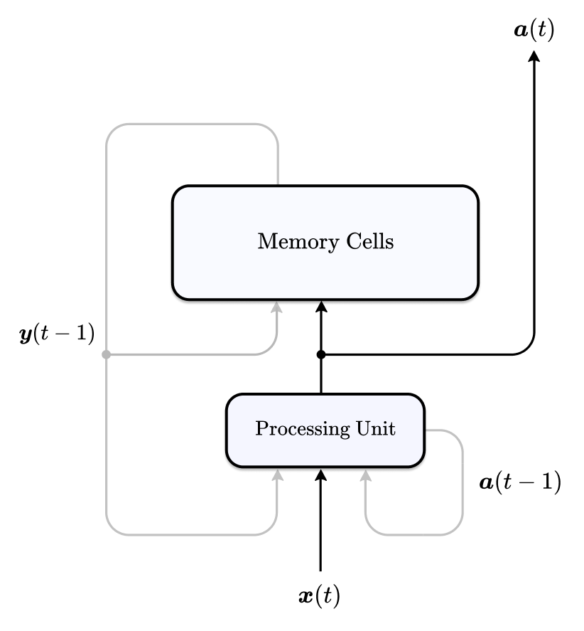
Figure 6: Schematic of LSTM with compute and memory decoupled.
The architecture is characterised by two main components – the processing unit and the memory cells. The memory consists of a cell state gated by an input and output gate and the processing unit is defined as a fully-recurrent layer with read access to the previous memory cell state activation \(\boldsymbol{y}(t-1)\). The old memory contents, external inputs \(\boldsymbol{x}(t)\) and its previous hidden activations \(\boldsymbol{a}(t-1)\) are used to compute the processing unit’s state \(\boldsymbol{a}(t)\). Based on this information, activations for the gates \(\boldsymbol{i}(t), \boldsymbol{o}(t)\) and cell input \(\boldsymbol{z}(t)\) of the memory are determined and results from the computational layer are stored within the memory cells for later use (write access).
Mathematically, we can define the architecture as follows:
\[ \begin{aligned} \boldsymbol{a}(t) &=f\left(\boldsymbol{W}_{a}^{\top} \boldsymbol{x}(t)+\boldsymbol{R}_{a}^{\top} \boldsymbol{a}(t-1)+\boldsymbol{U}_{a}^{\top} \boldsymbol{y}(t-1)\right) \\ \boldsymbol{i}(t) &=\sigma\left(\boldsymbol{W}_{i}^{\top} \boldsymbol{a}(t)+\boldsymbol{R}_{i}^{\top} \boldsymbol{y}(t-1)\right) \\ \boldsymbol{o}(t) &=\sigma\left(\boldsymbol{W}_{o}^{\top} \boldsymbol{a}(t)+\boldsymbol{R}_{o}^{\top} \boldsymbol{y}(t-1)\right) \\ \boldsymbol{z}(t) &=g\left(\boldsymbol{W}_{z}^{\top} \boldsymbol{a}(t)+\boldsymbol{R}_{z}^{\top} \boldsymbol{y}(t-1)\right) \\ \boldsymbol{c}(t) &=\boldsymbol{c}(t-1)+\boldsymbol{i}(t) \odot \boldsymbol{z}(t) \\ \boldsymbol{y}(t) &=\boldsymbol{o}(t) \odot h(\boldsymbol{c}(t)) \end{aligned} \]
Note that, instead of \(\boldsymbol{y}(t))\), we use \(\boldsymbol{a}(t)\), as the network’s output at time \(t\). In this way, inputs and outputs are connected exclusively to the processing layer. This wiring discourages the memory and processing unit from competing during the learning process as the main information stream flows through the fully-recurrent layer only. The processing module will initially try to solve the task on its own. However, when long-term dependencies need to be captured to solve the task, the network is forced to leverage the memory mechanisms. It will learn how to control the memory cells such that it can retain relevant information and retrieve it when necessary.
Chicken and Egg, online learning and more cells than necessary
Often when we train Recurrent Neural Networks, we are confronted with a Chicken-or-Egg-type dilemma: if, on the one hand, we start training with a good pattern detector that is able to extract relevant information from the input, we only need to learn appropriate storage mechanisms to retain the detected patterns. On the other hand, if we have the means of storing patterns, we only need to learn to extract the right ones from the input sequence. If neither is given, learning does not work – why learn storage mechanisms when we have no way to detect patterns? Why learn a good pattern detector when the detected patterns cannot be stored?
Fortunately, a good parameter initialisation usually gives us a solid initial guess for one or the other. This is often sufficient to instantiate a healthy error flow within the network and eventually enables it to master both the detection and storage of relevant patterns.
There are two ways how we can increase our chances of finding a good set of weights which parametrise the LSTM to either store or produce relevant input activations. First, in many cases learning can be sped up by updating the LSTM after each sequence as opposed to a batch of sequences. The frequent weight updates have an exploratory effect and are especially beneficial in the early stages of training. Second, simply use more cells than necessary! More cells increase our odds of instantiating a good detector whose activations are close to relevant patterns and storage mechanisms can be learned right away or vice versa.
Sequence classification vs. continuous prediction
Instead of continuously emitting a prediction at every time step, it can be advantageous to predict a single target at the end of the sequence. In this way, the LSTM does not have to trade off memory capacity and only has to store information that is relevant for the final output. Continous predictions can lead to high errors in situations where the targets can hardly be predicted (e.g. due to high variance). This can be detrimental to learning6.
Parallel LSTM networks for continuous prediction
An alternative approach is to bundle multiple LSTMs together in a parallel fashion. Each of the LSTMs is shifted by one time step and is tasked to predict a single target from a subsequence. As soon as a network has emitted a prediction, it can immediately be used again to process the next inputs – the computations can be parallelised across multiple workers.
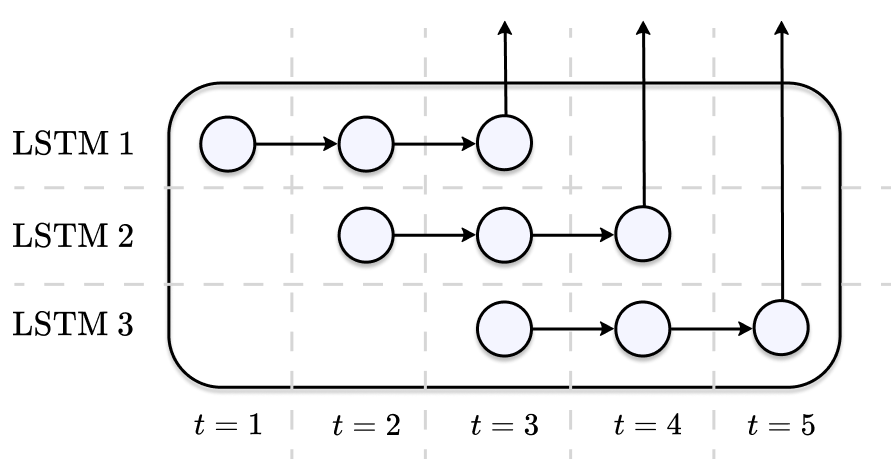
Figure 7: Continous prediction with multiple LSTMs. Each network receives sequences of length 3 and predicts a single target.
Because each network can focus on storing relevant patterns for a single prediction, we can usually do away with the forget gate and the output gate. This reduces the computational footprint of our parallel training scheme.
Target and input scaling
It is a good idea to rescale the targets into the range \([0.2, 0.8]\) when using sigmoid output units. This prevents the output activations from being pushed into saturated regions where learning stalls, i.e. zero gradients.
Always standardise the input to zero mean and unit variance. A neat trick you can use if there are outliers in the data is to standardise, apply tanh and then standardise again. Repeat this procedure to move the outliers closer towards the remaining data points. In this way, we can reduce the impact of outliers without entirely removing them.
A. Arjona-Medina, Jose, Michael Gillhofer, Michael Widrich, Thomas Unterthiner, Johannes Brandstetter, and Sepp Hochreiter. 2018. “RUDDER: Return Decomposition for Delayed Rewards.” http://arxiv.org/abs/1806.07857.
Gers, Felix A, Jürgen Schmidhuber, and Fred Cummins. 1999. “Learning to Forget: Continual Prediction with Lstm.”
Graves, Alex. 2016. “Adaptive Computation Time for Recurrent Neural Networks.” http://arxiv.org/abs/1603.08983.
Graves, Alex, Greg Wayne, and Ivo Danihelka. 2014. “Neural Turing Machines.” http://arxiv.org/abs/1410.5401.
Greff, Klaus, Rupesh K. Srivastava, Jan Koutnik, Bas R. Steunebrink, and Jurgen Schmidhuber. 2017. “LSTM: A Search Space Odyssey.” IEEE Transactions on Neural Networks and Learning Systems 28 (10): 2222–32. https://doi.org/10.1109/tnnls.2016.2582924.
Hafner, Danijar. 2017. “Tips for Training Recurrent Neural Networks.” Blog post. https://danijar.com/tips-for-training-recurrent-neural-networks/.
Hochreiter, Sepp, Martin Heusel, and Klaus Obermayer. 2007. “Fast Model-Based Protein Homology Detection Without Alignment.” Bioinformatics 23 (14): 1728–36.
Hochreiter, Sepp, and Jürgen Schmidhuber. 1997. “Long Short-Term Memory.” Neural Computation 9 (8): 1735–80.
Hochreiter, Sepp, A Steven Younger, and Peter R Conwell. 2001. “Learning to Learn Using Gradient Descent.” In International Conference on Artificial Neural Networks, 87–94. Springer.
Note that we omit the forget gate. The equation represents the cell state update used in the original LSTM paper.↩︎
This formulation is used in Gated Recurrent Units or GRUs.↩︎
Note, however, that this redundancy might not necessarily be bad since it increases the representational power of the network. Because of the symmetry between \(\boldsymbol{i}\) and \(\boldsymbol{z}\), the network has the flexibility to use either one of them, and we effectively doubled our chance of initialising a successful pattern detector.↩︎
If you observe oscillations, try removing the output gate or the forget gate.↩︎
Even though this behaviour is undesirable, it does lead to a certain degree of time awareness as the cell state is usually larger at later points in time.↩︎
See, for example, RUDDER (A. Arjona-Medina et al. 2018), where return predictions at the end of an episode were superior to trying to predict the reward continuously.↩︎